|
IMEXSfloW
1.0
templategithubproject
|
|
IMEXSfloW
1.0
templategithubproject
|
Numerical solver. More...
Public Member Functions | |
| subroutine | allocate_solver_variables |
| Memory allocation. More... | |
| subroutine | deallocate_solver_variables |
| Memory deallocation. More... | |
| subroutine | timestep |
| Time-step computation. More... | |
| subroutine | imex_rk_solver |
| Runge-Kutta integration. More... | |
| subroutine | solve_rk_step (Bj, Bprimej, qj, qj_old, a_tilde, a_dirk, a_diag) |
| Runge-Kutta single step integration. More... | |
| subroutine | lnsrch (Bj, Bprimej, qj_rel_NR_old, qj_org, qj_old, scal_f_old, grad_f, desc_dir, coeff_f, qj_rel, scal_f, right_term, stpmax, check) |
| Search the descent stepsize. More... | |
| subroutine | eval_f (Bj, Bprimej, qj, qj_old, a_tilde, a_dirk, a_diag, coeff_f, f_nl, scal_f) |
| Evaluate the nonlinear system. More... | |
| subroutine | eval_jacobian (Bj, Bprimej, qj_rel, qj_org, coeff_f, left_matrix) |
| Evaluate the jacobian. More... | |
| subroutine | eval_explicit_terms (q_expl, expl_terms) |
| Evaluate the explicit terms. More... | |
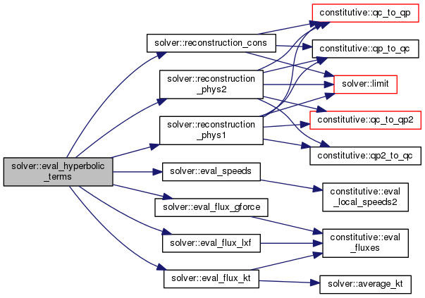
| subroutine | eval_hyperbolic_terms (q_expl, F_x) |
| Semidiscrete finite volume central scheme. More... | |
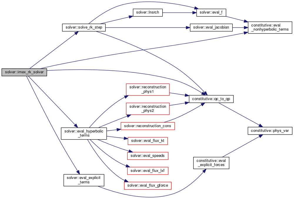
| subroutine | eval_flux_kt |
| Semidiscrete numerical fluxes. More... | |
| subroutine | average_kt (aL, aR, wL, wR, w_avg) |
| subroutine | eval_flux_gforce |
| Numerical fluxes GFORCE. More... | |
| subroutine | eval_flux_lxf |
| Numerical fluxes Lax-Friedrichs. More... | |
| subroutine | reconstruction_cons |
| Linear reconstruction. More... | |
| subroutine | reconstruction_phys1 |
| Linear reconstruction. More... | |
| subroutine | reconstruction_phys2 |
| Linear reconstruction. More... | |
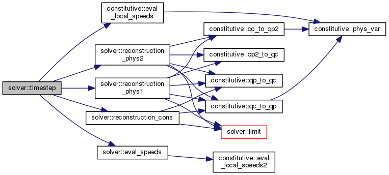
| subroutine | eval_speeds |
| Characteristic speeds. More... | |
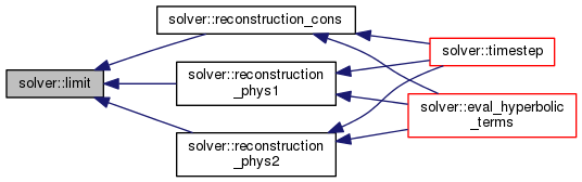
| subroutine | limit (v, z, limiter, slope_lim) |
| Slope limiter. More... | |
| real *8 function | minmod (a, b) |
| real *8 function | maxmod (a, b) |
Public Attributes | |
| real *8, dimension(:,:), allocatable | q |
| Conservative variables. More... | |
| real *8, dimension(:,:), allocatable | q0 |
| Conservative variables. More... | |
| real *8, dimension(:,:), allocatable | q_fv |
| Solution of the finite-volume semidiscrete cheme. More... | |
| real *8, dimension(:,:), allocatable | q_interfacel |
| Reconstructed value at the left of the interface. More... | |
| real *8, dimension(:,:), allocatable | q_interfacer |
| Reconstructed value at the right of the interface. More... | |
| real *8, dimension(:,:), allocatable | a_interfacel |
| Local speeds at the left of the interface. More... | |
| real *8, dimension(:,:), allocatable | a_interfacer |
| Local speeds at the right of the interface. More... | |
| real *8, dimension(:,:), allocatable | h_interface |
| Semidiscrete numerical interface fluxes. More... | |
| real *8, dimension(:,:), allocatable | qp |
Physical variables (  ) More... ) More... | |
| real *8 | dt |
| Time step. More... | |
| logical, dimension(:,:), allocatable | mask22 |
| logical, dimension(:,:), allocatable | mask21 |
| logical, dimension(:,:), allocatable | mask11 |
| logical, dimension(:,:), allocatable | mask12 |
| real *8, dimension(:,:), allocatable | a_tilde_ij |
| Butcher Tableau for the explicit part of the Runge-Kutta scheme. More... | |
| real *8, dimension(:,:), allocatable | a_dirk_ij |
| Butcher Tableau for the implicit part of the Runge-Kutta scheme. More... | |
| real *8, dimension(:), allocatable | omega_tilde |
| Coefficients for the explicit part of the Runge-Kutta scheme. More... | |
| real *8, dimension(:), allocatable | omega |
| Coefficients for the implicit part of the Runge-Kutta scheme. More... | |
| real *8, dimension(:), allocatable | a_tilde |
| Explicit coefficients for the hyperbolic part for a single step of the R-K scheme. More... | |
| real *8, dimension(:), allocatable | a_dirk |
| Explicit coefficients for the non-hyperbolic part for a single step of the R-K scheme. More... | |
| real *8 | a_diag |
| Implicit coefficient for the non-hyperbolic part for a single step of the R-K scheme. More... | |
| real *8, dimension(:,:,:), allocatable | q_rk |
| Intermediate solutions of the Runge-Kutta scheme. More... | |
| real *8, dimension(:,:,:), allocatable | f_x |
| Intermediate hyperbolic terms of the Runge-Kutta scheme. More... | |
| real *8, dimension(:,:,:), allocatable | nh |
| Intermediate non-hyperbolic terms of the Runge-Kutta scheme. More... | |
| real *8, dimension(:,:,:), allocatable | expl_terms |
| Intermediate explicit terms of the Runge-Kutta scheme. More... | |
| real *8, dimension(:,:), allocatable | fxj |
| Local Intermediate hyperbolic terms of the Runge-Kutta scheme. More... | |
| real *8, dimension(:,:), allocatable | nhj |
| Local Intermediate non-hyperbolic terms of the Runge-Kutta scheme. More... | |
| real *8, dimension(:,:), allocatable | expl_terms_j |
| Local Intermediate explicit terms of the Runge-Kutta scheme. More... | |
| logical | normalize_q |
| logical | normalize_f |
| logical | opt_search_nl |
| real *8, dimension(:,:), allocatable | residual_term |
Numerical solver.
This module contains the variables and the subroutines for the numerical solution of the equations.
Definition at line 12 of file solver.f90.
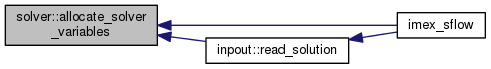
| subroutine solver::allocate_solver_variables | ( | ) |
Memory allocation.
This subroutine allocate the memory for the variables of the solver module.
Definition at line 112 of file solver.f90.
| subroutine solver::average_kt | ( | real*8, dimension(:), intent(in) | aL, |
| real*8, dimension(:), intent(in) | aR, | ||
| real*8, dimension(:), intent(in) | wL, | ||
| real*8, dimension(:), intent(in) | wR, | ||
| real*8, dimension(:), intent(out) | w_avg | ||
| ) |
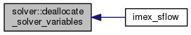
| subroutine solver::deallocate_solver_variables | ( | ) |
Memory deallocation.
This subroutine de-allocate the memory for the variables of the solver module.
Definition at line 270 of file solver.f90.
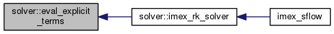
| subroutine solver::eval_explicit_terms | ( | real*8, dimension(n_vars,comp_cells), intent(in) | q_expl, |
| real*8, dimension(n_eqns,comp_cells), intent(out) | expl_terms | ||
| ) |
Evaluate the explicit terms.
This subroutine evaluate the explicit terms (non-fluxes) of the non-linear system with respect to the conservative variables.
| [in] | q_expl | conservative variables |
| [out] | expl_terms | explicit terms |
Definition at line 1265 of file solver.f90.

| subroutine solver::eval_f | ( | real*8, intent(in) | Bj, |
| real*8, intent(in) | Bprimej, | ||
| real*8, dimension(n_vars), intent(in) | qj, | ||
| real*8, dimension(n_vars), intent(in) | qj_old, | ||
| real*8, dimension(n_rk), intent(in) | a_tilde, | ||
| real*8, dimension(n_rk), intent(in) | a_dirk, | ||
| real*8, intent(in) | a_diag, | ||
| real*8, dimension(n_eqns), intent(in) | coeff_f, | ||
| real*8, dimension(n_eqns), intent(out) | f_nl, | ||
| real*8, intent(out) | scal_f | ||
| ) |
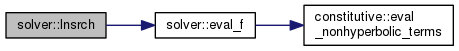
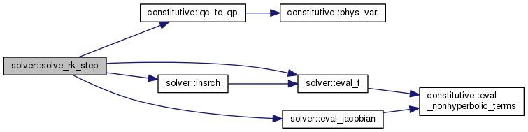
Evaluate the nonlinear system.
This subroutine evaluate the value of the nonlinear system in the state defined by the variables qj.
| [in] | Bj | batimetry at the cell center |
| [in] | Bprimej | batimetry slope at the cell center |
| [in] | qj | conservative variables |
| [in] | qj_old | conservative variables at the old time step |
| [in] | a_tilde | explicit coefficients for the hyperbolic terms |
| [in] | a_dirk | explicit coefficients for the non-hyperbolic terms |
| [in] | a_diag | implicit coefficient for the non-hyperbolic term |
| [in] | coeff_f | coefficient to rescale the nonlinear functions |
| [out] | f_nl | values of the nonlinear functions |
| [out] | scal_f | value of the scalar function f=0.5*<F,F> |
Definition at line 1145 of file solver.f90.

| subroutine solver::eval_flux_gforce | ( | ) |
Numerical fluxes GFORCE.
Definition at line 1536 of file solver.f90.

| subroutine solver::eval_flux_kt | ( | ) |
Semidiscrete numerical fluxes.
This subroutine evaluates the numerical fluxes H at the cells interfaces according to Kurganov et al. 2001.
Definition at line 1428 of file solver.f90.

| subroutine solver::eval_flux_lxf | ( | ) |
Numerical fluxes Lax-Friedrichs.
Definition at line 1605 of file solver.f90.

| subroutine solver::eval_hyperbolic_terms | ( | real*8, dimension(n_vars,comp_cells), intent(in) | q_expl, |
| real*8, dimension(n_eqns,comp_cells), intent(out) | F_x | ||
| ) |
Semidiscrete finite volume central scheme.
This subroutine solve the hyperbolic part of the system of the eqns, with a modified finite volume scheme from Kurganov et al. 2001, coupled with a MUSCL-Hancock scheme (Van Leer, 1984) applied to a set of physical variables derived from the conservative vriables.
Definition at line 1303 of file solver.f90.
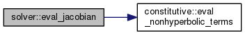
| subroutine solver::eval_jacobian | ( | real*8, intent(in) | Bj, |
| real*8, intent(in) | Bprimej, | ||
| real*8, dimension(n_vars), intent(in) | qj_rel, | ||
| real*8, dimension(n_vars), intent(in) | qj_org, | ||
| real*8, dimension(n_eqns), intent(in) | coeff_f, | ||
| real*8, dimension(n_eqns,n_vars), intent(out) | left_matrix | ||
| ) |
Evaluate the jacobian.
This subroutine evaluate the jacobian of the non-linear system with respect to the conservative variables.
| [in] | Bj | batimetry at the cell center |
| [in] | Bprimej | batimetry slope at the cell center |
| [in] | qj_rel | relative variation (qj=qj_rel*qj_org) |
| [in] | qj_org | conservative variables at the old time step |
| [in] | coeff_f | coefficient to rescale the nonlinear functions |
| [out] | left_matrix | matrix from the linearization of the system |
Definition at line 1197 of file solver.f90.

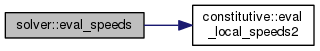
| subroutine solver::eval_speeds | ( | ) |
Characteristic speeds.
This subroutine evaluates the largest characteristic speed at the cells interfaces from the reconstructed states.
Definition at line 2553 of file solver.f90.
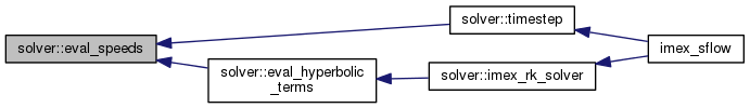
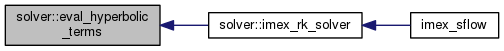
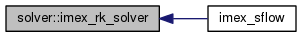
| subroutine solver::imex_rk_solver | ( | ) |
Runge-Kutta integration.
This subroutine integrate the hyperbolic conservation law with non-hyperbolic terms using an implicit-explicit runge-kutta scheme. The fluxes are integrated explicitely while the non-hyperbolic terms are integrated implicitely.
Definition at line 414 of file solver.f90.
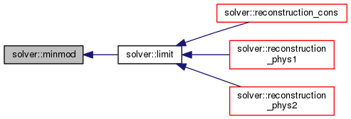
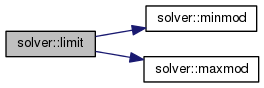
| subroutine solver::limit | ( | real*8, dimension(3), intent(in) | v, |
| real*8, dimension(3), intent(in) | z, | ||
| integer, intent(in) | limiter, | ||
| real*8, intent(out) | slope_lim | ||
| ) |
Slope limiter.
This subroutine limits the slope of the linear reconstruction of the physical variables, accordingly to the parameter "solve_limiter":
| [in] | v | 3-point stencil value array |
| [in] | z | 3-point stencil location array |
| [out] | slope_lim | limited slope |
Definition at line 2603 of file solver.f90.
| subroutine solver::lnsrch | ( | real*8, intent(in) | Bj, |
| real*8, intent(in) | Bprimej, | ||
| real*8, dimension(:), intent(in) | qj_rel_NR_old, | ||
| real*8, dimension(:), intent(in) | qj_org, | ||
| real*8, dimension(:), intent(in) | qj_old, | ||
| real*8, intent(in) | scal_f_old, | ||
| real*8, dimension(:), intent(in) | grad_f, | ||
| real*8, dimension(:), intent(inout) | desc_dir, | ||
| real*8, dimension(:), intent(in) | coeff_f, | ||
| real*8, dimension(:), intent(out) | qj_rel, | ||
| real*8, intent(out) | scal_f, | ||
| real*8, dimension(n_eqns), intent(out) | right_term, | ||
| real*8, intent(in) | stpmax, | ||
| logical, intent(out) | check | ||
| ) |
Search the descent stepsize.
This subroutine search for the lenght of the descent step in order to have a decrease in the nonlinear function.
| [in] | Bj | batimetry at the cell center |
| [in] | Bprimej | batimetry slope at the cell center |
| [in] | qj_rel_NR_old | |
| [in] | qj_org | |
| [in] | qj_old | |
| [in] | scal_f_old | |
| [in] | grad_f | |
| [in,out] | desc_dir | |
| [in] | coeff_f | |
| [out] | qj_rel | |
| [out] | scal_f | |
| [out] | right_term | |
| [in] | stpmax | |
| [out] | check |
| [in] | qj_rel_nr_old | Initial point |
| [in] | qj_org | Initial point |
| [in] | qj_old | Initial point |
| [in] | grad_f | Gradient at xold |
| [in] | scal_f_old | Value of the function at xold |
| [in,out] | desc_dir | Descent direction (usually Newton direction) |
| [in] | coeff_f | Coefficients to rescale the nonlinear function |
| [out] | qj_rel | Updated solution |
| [out] | scal_f | Value of the scalar function at x |
| [out] | right_term | Value of the scalar function at x |
| [out] | check | Output quantity check is false on a normal exit |
Definition at line 924 of file solver.f90.

| real*8 function solver::maxmod | ( | real*8 | a, |
| real*8 | b | ||
| ) |
| real*8 function solver::minmod | ( | real*8 | a, |
| real*8 | b | ||
| ) |
| subroutine solver::reconstruction_cons | ( | ) |
Linear reconstruction.
In this subroutine a linear reconstruction with slope limiters is applied to a set of conservative variables describing the state of the system.
Definition at line 1664 of file solver.f90.


| subroutine solver::reconstruction_phys1 | ( | ) |
Linear reconstruction.
In this subroutine a linear reconstruction with slope limiters is applied to a set of physical variables (h+B,u) describing the state of the system.
Definition at line 1950 of file solver.f90.


| subroutine solver::reconstruction_phys2 | ( | ) |
Linear reconstruction.
In this subroutine a linear reconstruction with slope limiters is applied to a set of physical variables (h,u) describing the state of the system.
Definition at line 2252 of file solver.f90.


| subroutine solver::solve_rk_step | ( | real*8, intent(in) | Bj, |
| real*8, intent(in) | Bprimej, | ||
| real*8, dimension(n_vars), intent(inout) | qj, | ||
| real*8, dimension(n_vars), intent(in) | qj_old, | ||
| real*8, dimension(n_rk), intent(in) | a_tilde, | ||
| real*8, dimension(n_rk), intent(in) | a_dirk, | ||
| real*8, intent(in) | a_diag | ||
| ) |
Runge-Kutta single step integration.
This subroutine find the solution of the non-linear system given the a step of the implicit-explicit Runge-Kutta scheme for a cell:

| [in] | Bj | batimetry at the cell center |
| [in] | Bprimej | batimetry slope at the cell center |
| [in,out] | qj | conservative variables |
| [in] | qj_old | conservative variables at the old time step |
| [in] | a_tilde | explicit coefficents for the fluxes |
| [in] | a_dirk | explicit coefficient for the non-hyperbolic terms |
| [in] | a_diag | implicit coefficient for the non-hyperbolic terms |
Definition at line 605 of file solver.f90.

| subroutine solver::timestep | ( | ) |
Time-step computation.
This subroutine evaluate the maximum time step according to the CFL condition. The local speed are evaluated with the characteristic polynomial of the Jacobian of the fluxes.
Definition at line 322 of file solver.f90.
| real*8 solver::a_diag |
Implicit coefficient for the non-hyperbolic part for a single step of the R-K scheme.
Definition at line 72 of file solver.f90.
| real*8, dimension(:), allocatable solver::a_dirk |
Explicit coefficients for the non-hyperbolic part for a single step of the R-K scheme.
Definition at line 70 of file solver.f90.
| real*8, dimension(:,:), allocatable solver::a_dirk_ij |
Butcher Tableau for the implicit part of the Runge-Kutta scheme.
Definition at line 60 of file solver.f90.
| real*8, dimension(:,:), allocatable solver::a_interfacel |
Local speeds at the left of the interface.
Definition at line 43 of file solver.f90.
| real*8, dimension(:,:), allocatable solver::a_interfacer |
Local speeds at the right of the interface.
Definition at line 45 of file solver.f90.
| real*8, dimension(:), allocatable solver::a_tilde |
Explicit coefficients for the hyperbolic part for a single step of the R-K scheme.
Definition at line 68 of file solver.f90.
| real*8, dimension(:,:), allocatable solver::a_tilde_ij |
Butcher Tableau for the explicit part of the Runge-Kutta scheme.
Definition at line 58 of file solver.f90.
| real*8 solver::dt |
Time step.
Definition at line 53 of file solver.f90.
| real*8, dimension(:,:,:), allocatable solver::expl_terms |
Intermediate explicit terms of the Runge-Kutta scheme.
Definition at line 82 of file solver.f90.
| real*8, dimension(:,:), allocatable solver::expl_terms_j |
Local Intermediate explicit terms of the Runge-Kutta scheme.
Definition at line 89 of file solver.f90.
| real*8, dimension(:,:,:), allocatable solver::f_x |
Intermediate hyperbolic terms of the Runge-Kutta scheme.
Definition at line 77 of file solver.f90.
| real*8, dimension(:,:), allocatable solver::fxj |
Local Intermediate hyperbolic terms of the Runge-Kutta scheme.
Definition at line 85 of file solver.f90.
| real*8, dimension(:,:), allocatable solver::h_interface |
Semidiscrete numerical interface fluxes.
Definition at line 47 of file solver.f90.
| logical, dimension(:,:), allocatable solver::mask11 |
Definition at line 55 of file solver.f90.
| logical, dimension(:,:), allocatable solver::mask12 |
Definition at line 55 of file solver.f90.
| logical, dimension(:,:), allocatable solver::mask21 |
Definition at line 55 of file solver.f90.
| logical, dimension(:,:), allocatable solver::mask22 |
Definition at line 55 of file solver.f90.
| real*8, dimension(:,:,:), allocatable solver::nh |
Intermediate non-hyperbolic terms of the Runge-Kutta scheme.
Definition at line 79 of file solver.f90.
| real*8, dimension(:,:), allocatable solver::nhj |
Local Intermediate non-hyperbolic terms of the Runge-Kutta scheme.
Definition at line 87 of file solver.f90.
| logical solver::normalize_f |
Definition at line 92 of file solver.f90.
| logical solver::normalize_q |
Definition at line 91 of file solver.f90.
| real*8, dimension(:), allocatable solver::omega |
Coefficients for the implicit part of the Runge-Kutta scheme.
Definition at line 65 of file solver.f90.
| real*8, dimension(:), allocatable solver::omega_tilde |
Coefficients for the explicit part of the Runge-Kutta scheme.
Definition at line 63 of file solver.f90.
| logical solver::opt_search_nl |
Definition at line 93 of file solver.f90.
| real*8, dimension(:,:), allocatable solver::q |
Conservative variables.
Definition at line 33 of file solver.f90.
| real*8, dimension(:,:), allocatable solver::q0 |
Conservative variables.
Definition at line 35 of file solver.f90.
| real*8, dimension(:,:), allocatable solver::q_fv |
Solution of the finite-volume semidiscrete cheme.
Definition at line 37 of file solver.f90.
| real*8, dimension(:,:), allocatable solver::q_interfacel |
Reconstructed value at the left of the interface.
Definition at line 39 of file solver.f90.
| real*8, dimension(:,:), allocatable solver::q_interfacer |
Reconstructed value at the right of the interface.
Definition at line 41 of file solver.f90.
| real*8, dimension(:,:,:), allocatable solver::q_rk |
Intermediate solutions of the Runge-Kutta scheme.
Definition at line 75 of file solver.f90.
| real*8, dimension(:,:), allocatable solver::qp |
Physical variables ( )
Definition at line 49 of file solver.f90.
| real*8, dimension(:,:), allocatable solver::residual_term |
Definition at line 95 of file solver.f90.
 1.8.7
1.8.7