|
SW_VAR_DENS_MODEL
0.9
Dept-averagedgas-particlemodel
|
Numerical solver. More...
Functions/Subroutines | |
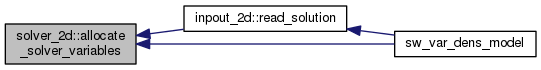
| subroutine | allocate_solver_variables |
| Memory allocation. More... | |
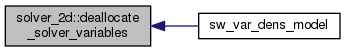
| subroutine | deallocate_solver_variables |
| Memory deallocation. More... | |
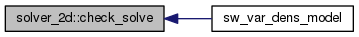
| subroutine | check_solve |
| Masking of cells to solve. More... | |
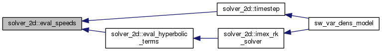
| subroutine | timestep |
| Time-step computation. More... | |
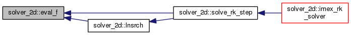
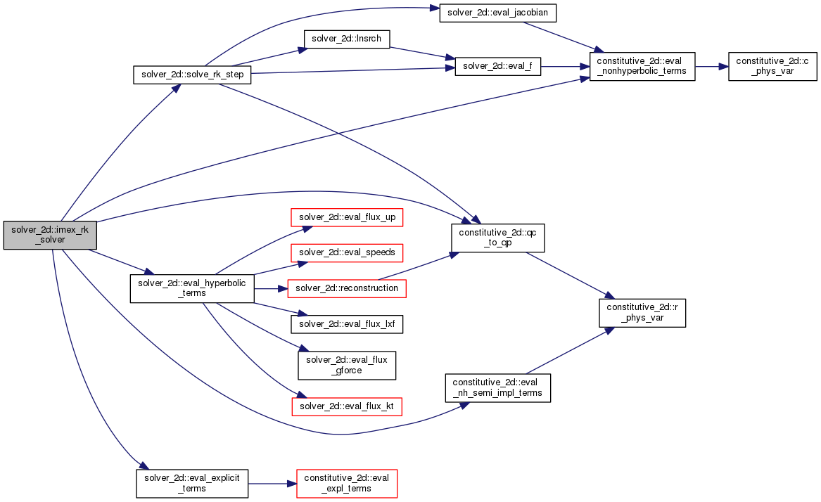
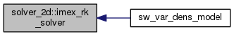
| subroutine | imex_rk_solver |
| Runge-Kutta integration. More... | |
| subroutine | solve_rk_step (qj, qj_old, a_tilde, a_dirk, a_diag) |
| Runge-Kutta single step integration. More... | |
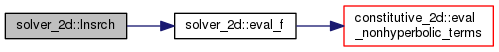
| subroutine | lnsrch (qj_rel_NR_old, qj_org, qj_old, scal_f_old, grad_f, desc_dir, coeff_f, qj_rel, scal_f, right_term, stpmax, check) |
| Search the descent stepsize. More... | |
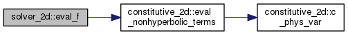
| subroutine | eval_f (qj, qj_old, a_tilde, a_dirk, a_diag, coeff_f, f_nl, scal_f) |
| Evaluate the nonlinear system. More... | |
| subroutine | eval_jacobian (qj_rel, qj_org, coeff_f, left_matrix) |
| Evaluate the jacobian. More... | |
| subroutine | update_erosion_deposition_cell (dt) |
| Evaluate the eroion/deposition terms. More... | |
| subroutine | eval_explicit_terms (qc_expl, qp_expl, expl_terms) |
| Evaluate the explicit terms. More... | |
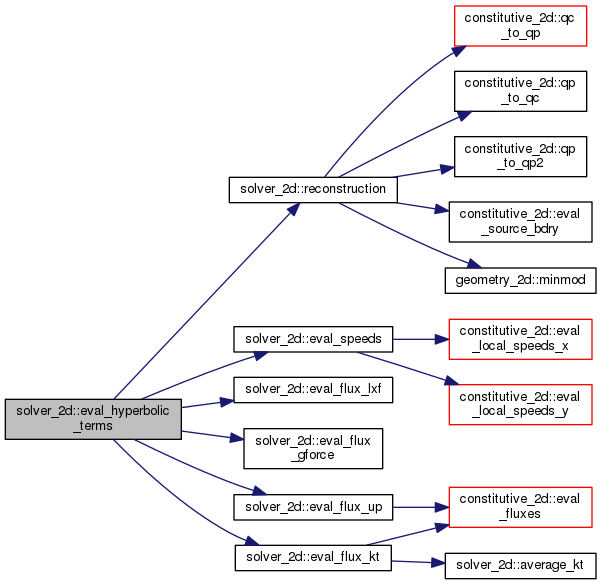
| subroutine | eval_hyperbolic_terms (q_expl, qp_expl, divFlux) |
| Semidiscrete finite volume central scheme. More... | |
| subroutine | eval_flux_up |
| Upwind numerical fluxes. More... | |
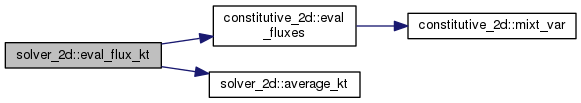
| subroutine | eval_flux_kt |
| Semidiscrete numerical fluxes. More... | |
| subroutine | average_kt (a1, a2, w1, w2, w_avg) |
| averaged KT flux More... | |
| subroutine | eval_flux_gforce |
| Numerical fluxes GFORCE. More... | |
| subroutine | eval_flux_lxf |
| Numerical fluxes Lax-Friedrichs. More... | |
| subroutine | reconstruction (q_expl, qp_expl) |
| Linear reconstruction. More... | |
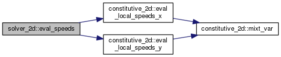
| subroutine | eval_speeds |
| Characteristic speeds. More... | |
Variables | |
| real *8 | t |
| time More... | |
| real *8, dimension(:,:,:), allocatable | q |
| Conservative variables. More... | |
| real *8, dimension(:,:,:), allocatable | q0 |
| Conservative variables. More... | |
| real *8, dimension(:,:,:), allocatable | q_fv |
| Solution of the finite-volume semidiscrete cheme. More... | |
| real *8, dimension(:,:,:), allocatable | q_interfacel |
| Reconstructed value at the left of the x-interface. More... | |
| real *8, dimension(:,:,:), allocatable | q_interfacer |
| Reconstructed value at the right of the x-interface. More... | |
| real *8, dimension(:,:,:), allocatable | q_interfaceb |
| Reconstructed value at the bottom of the y-interface. More... | |
| real *8, dimension(:,:,:), allocatable | q_interfacet |
| Reconstructed value at the top of the y-interface. More... | |
| real *8, dimension(:,:,:), allocatable | qp_interfacel |
| Reconstructed physical value at the left of the x-interface. More... | |
| real *8, dimension(:,:,:), allocatable | qp_interfacer |
| Reconstructed physical value at the right of the x-interface. More... | |
| real *8, dimension(:,:,:), allocatable | qp_interfaceb |
| Reconstructed physical value at the bottom of the y-interface. More... | |
| real *8, dimension(:,:,:), allocatable | qp_interfacet |
| Reconstructed physical value at the top of the y-interface. More... | |
| real *8, dimension(:,:,:), allocatable | q_cellnw |
| Reconstructed value at the NW corner of cell. More... | |
| real *8, dimension(:,:,:), allocatable | q_cellne |
| Reconstructed value at the NE corner of cell. More... | |
| real *8, dimension(:,:,:), allocatable | q_cellsw |
| Reconstructed value at the SW corner of cell. More... | |
| real *8, dimension(:,:,:), allocatable | q_cellse |
| Reconstructed value at the SE corner of cell. More... | |
| real *8, dimension(:,:,:), allocatable | qp_cellnw |
| Reconstructed physical value at the NW corner of cell. More... | |
| real *8, dimension(:,:,:), allocatable | qp_cellne |
| Reconstructed physical value at the NE corner of cell. More... | |
| real *8, dimension(:,:,:), allocatable | qp_cellsw |
| Reconstructed physical value at the SW corner of cell. More... | |
| real *8, dimension(:,:,:), allocatable | qp_cellse |
| Reconstructed physical value at the SE corner of cell. More... | |
| real *8, dimension(:,:), allocatable | q1max |
| Maximum over time of thickness. More... | |
| real *8, dimension(:,:,:), allocatable | a_interface_x_max |
| Max local speeds at the x-interface. More... | |
| real *8, dimension(:,:,:), allocatable | a_interface_y_max |
| Max local speeds at the y-interface. More... | |
| real *8, dimension(:,:,:), allocatable | a_interface_xneg |
| Local speeds at the left of the x-interface. More... | |
| real *8, dimension(:,:,:), allocatable | a_interface_xpos |
| Local speeds at the right of the x-interface. More... | |
| real *8, dimension(:,:,:), allocatable | a_interface_yneg |
| Local speeds at the bottom of the y-interface. More... | |
| real *8, dimension(:,:,:), allocatable | a_interface_ypos |
| Local speeds at the top of the y-interface. More... | |
| real *8, dimension(:,:,:), allocatable | h_interface_x |
| Semidiscrete numerical interface fluxes. More... | |
| real *8, dimension(:,:,:), allocatable | h_interface_y |
| Semidiscrete numerical interface fluxes. More... | |
| real *8, dimension(:,:,:), allocatable | qp |
Physical variables (  ) More... ) More... | |
| real *8, dimension(:,:), allocatable | source_xy |
| Array defining fraction of cells affected by source term. More... | |
| logical, dimension(:,:), allocatable | solve_mask |
| logical, dimension(:,:), allocatable | solve_mask_x |
| logical, dimension(:,:), allocatable | solve_mask_y |
| integer | solve_cells |
| integer | solve_interfaces_x |
| integer | solve_interfaces_y |
| real *8 | dt |
| Time step. More... | |
| logical, dimension(:,:), allocatable | mask22 |
| logical, dimension(:,:), allocatable | mask21 |
| logical, dimension(:,:), allocatable | mask11 |
| logical, dimension(:,:), allocatable | mask12 |
| integer | i_rk |
| loop counter for the RK iteration More... | |
| real *8, dimension(:,:), allocatable | a_tilde_ij |
| Butcher Tableau for the explicit part of the Runge-Kutta scheme. More... | |
| real *8, dimension(:,:), allocatable | a_dirk_ij |
| Butcher Tableau for the implicit part of the Runge-Kutta scheme. More... | |
| real *8, dimension(:), allocatable | omega_tilde |
| Coefficients for the explicit part of the Runge-Kutta scheme. More... | |
| real *8, dimension(:), allocatable | omega |
| Coefficients for the implicit part of the Runge-Kutta scheme. More... | |
| real *8, dimension(:), allocatable | a_tilde |
| Explicit coeff. for the hyperbolic part for a single step of the R-K scheme. More... | |
| real *8, dimension(:), allocatable | a_dirk |
| Explicit coeff. for the non-hyp. part for a single step of the R-K scheme. More... | |
| real *8 | a_diag |
| Implicit coeff. for the non-hyp. part for a single step of the R-K scheme. More... | |
| real *8, dimension(:,:,:,:), allocatable | q_rk |
| Intermediate solutions of the Runge-Kutta scheme. More... | |
| real *8, dimension(:,:,:,:), allocatable | qp_rk |
| Intermediate physical solutions of the Runge-Kutta scheme. More... | |
| real *8, dimension(:,:,:,:), allocatable | divflux |
| Intermediate hyperbolic terms of the Runge-Kutta scheme. More... | |
| real *8, dimension(:,:,:,:), allocatable | nh |
| Intermediate non-hyperbolic terms of the Runge-Kutta scheme. More... | |
| real *8, dimension(:,:,:,:), allocatable | si_nh |
| Intermediate semi-implicit non-hyperbolic terms of the Runge-Kutta scheme. More... | |
| real *8, dimension(:,:,:,:), allocatable | expl_terms |
| Intermediate explicit terms of the Runge-Kutta scheme. More... | |
| real *8, dimension(:,:), allocatable | divfluxj |
| Local Intermediate hyperbolic terms of the Runge-Kutta scheme. More... | |
| real *8, dimension(:,:), allocatable | nhj |
| Local Intermediate non-hyperbolic terms of the Runge-Kutta scheme. More... | |
| real *8, dimension(:,:), allocatable | expl_terms_j |
| Local Intermediate explicit terms of the Runge-Kutta scheme. More... | |
| real *8, dimension(:,:), allocatable | si_nhj |
| Local Intermediate semi-impl non-hyperbolic terms of the Runge-Kutta scheme. More... | |
| logical | normalize_q |
| Flag for the normalization of the array q in the implicit solution scheme. More... | |
| logical | normalize_f |
| Flag for the normalization of the array f in the implicit solution scheme. More... | |
| logical | opt_search_nl |
| Flag for the search of optimal step size in the implicit solution scheme. More... | |
| real *8, dimension(:,:,:), allocatable | residual_term |
| Sum of all the terms of the equations except the transient term. More... | |
| integer, dimension(:), allocatable | j_cent |
| integer, dimension(:), allocatable | k_cent |
| integer, dimension(:), allocatable | j_stag_x |
| integer, dimension(:), allocatable | k_stag_x |
| integer, dimension(:), allocatable | j_stag_y |
| integer, dimension(:), allocatable | k_stag_y |
| real *8 | t_imex1 |
| real *8 | t_imex2 |
Numerical solver.
This module contains the variables and the subroutines for the numerical solution of the equations.
| subroutine solver_2d::allocate_solver_variables | ( | ) |
Memory allocation.
This subroutine allocate the memory for the variables of the solver module.
Definition at line 216 of file solver_2d.f90.
| subroutine solver_2d::average_kt | ( | real*8, dimension(:), intent(in) | a1, |
| real*8, dimension(:), intent(in) | a2, | ||
| real*8, dimension(:), intent(in) | w1, | ||
| real*8, dimension(:), intent(in) | w2, | ||
| real*8, dimension(:), intent(out) | w_avg | ||
| ) |
averaged KT flux
This subroutine compute n averaged flux from the fluxes at the two sides of a cell interface and the max an min speed at the two sides.
| [in] | a1 | speed at one side of the interface |
| [in] | a2 | speed at the other side of the interface |
| [in] | w1 | fluxes at one side of the interface |
| [in] | w2 | fluxes at the other side of the interface |
| [out] | w_avg | array of averaged fluxes |
Definition at line 2410 of file solver_2d.f90.

| subroutine solver_2d::check_solve | ( | ) |
Masking of cells to solve.
This subroutine compute a 2D array of logicals defining the cells where the systems of equations have to be solved. It is defined according to the positive thickness in the cell and in the neighbour cells
Definition at line 548 of file solver_2d.f90.
| subroutine solver_2d::deallocate_solver_variables | ( | ) |
Memory deallocation.
This subroutine de-allocate the memory for the variables of the solver module.
Definition at line 452 of file solver_2d.f90.
| subroutine solver_2d::eval_explicit_terms | ( | real*8, dimension(n_vars,comp_cells_x,comp_cells_y), intent(in) | qc_expl, |
| real*8, dimension(n_vars+2,comp_cells_x,comp_cells_y), intent(in) | qp_expl, | ||
| real*8, dimension(n_eqns,comp_cells_x,comp_cells_y), intent(out) | expl_terms | ||
| ) |
Evaluate the explicit terms.
This subroutine evaluate the explicit terms (non-fluxes) of the non-linear system with respect to the conservative variables.
| [in] | qc_expl | conservative variables |
| [in] | qp_expl | conservative variables |
| [out] | expl_terms | explicit terms |
Definition at line 1999 of file solver_2d.f90.


| subroutine solver_2d::eval_f | ( | real*8, dimension(n_vars), intent(in) | qj, |
| real*8, dimension(n_vars), intent(in) | qj_old, | ||
| real*8, dimension(n_rk), intent(in) | a_tilde, | ||
| real*8, dimension(n_rk), intent(in) | a_dirk, | ||
| real*8, intent(in) | a_diag, | ||
| real*8, dimension(n_eqns), intent(in) | coeff_f, | ||
| real*8, dimension(n_eqns), intent(out) | f_nl, | ||
| real*8, intent(out) | scal_f | ||
| ) |
Evaluate the nonlinear system.
This subroutine evaluate the value of the nonlinear system in the state defined by the variables qj.
| [in] | qj | conservative variables |
| [in] | qj_old | conservative variables at the old time step |
| [in] | a_tilde | explicit coefficients for the hyperbolic terms |
| [in] | a_dirk | explicit coefficients for the non-hyperbolic terms |
| [in] | a_diag | implicit coefficient for the non-hyperbolic term |
| [in] | coeff_f | coefficient to rescale the nonlinear functions |
| [out] | f_nl | values of the nonlinear functions |
| [out] | scal_f | value of the scalar function f=0.5*<F,F> |
Definition at line 1759 of file solver_2d.f90.
| subroutine solver_2d::eval_flux_gforce | ( | ) |
Numerical fluxes GFORCE.
Definition at line 2449 of file solver_2d.f90.

| subroutine solver_2d::eval_flux_kt | ( | ) |
Semidiscrete numerical fluxes.
This subroutine evaluates the numerical fluxes H at the cells interfaces according to Kurganov et al. 2001.
Definition at line 2275 of file solver_2d.f90.

| subroutine solver_2d::eval_flux_lxf | ( | ) |
Numerical fluxes Lax-Friedrichs.
Definition at line 2463 of file solver_2d.f90.

| subroutine solver_2d::eval_flux_up | ( | ) |
Upwind numerical fluxes.
This subroutine evaluates the numerical fluxes H at the cells interfaces with an upwind discretization.
Definition at line 2157 of file solver_2d.f90.


| subroutine solver_2d::eval_hyperbolic_terms | ( | real*8, dimension(n_vars,comp_cells_x,comp_cells_y), intent(in) | q_expl, |
| real*8, dimension(n_vars+2,comp_cells_x,comp_cells_y), intent(in) | qp_expl, | ||
| real*8, dimension(n_eqns,comp_cells_x,comp_cells_y), intent(out) | divFlux | ||
| ) |
Semidiscrete finite volume central scheme.
This subroutine compute the divergence part of the system of the eqns, with a modified version of the finite volume scheme from Kurganov et al. 2001, where the reconstruction at the cells interfaces is applied to a set of physical variables derived from the conservative vriables.
| [in] | q_expl | conservative variables |
| [in] | qp_expl | conservative variables |
| [out] | divFlux | divergence term |
Definition at line 2053 of file solver_2d.f90.

| subroutine solver_2d::eval_jacobian | ( | real*8, dimension(n_vars), intent(in) | qj_rel, |
| real*8, dimension(n_vars), intent(in) | qj_org, | ||
| real*8, dimension(n_eqns), intent(in) | coeff_f, | ||
| real*8, dimension(n_eqns,n_vars), intent(out) | left_matrix | ||
| ) |
Evaluate the jacobian.
This subroutine evaluate the jacobian of the non-linear system with respect to the conservative variables.
| [in] | qj_rel | relative variation (qj=qj_rel*qj_org) |
| [in] | qj_org | conservative variables at the old time step |
| [in] | coeff_f | coefficient to rescale the nonlinear functions |
| [out] | left_matrix | matrix from the linearization of the system |
Definition at line 1810 of file solver_2d.f90.


| subroutine solver_2d::eval_speeds | ( | ) |
Characteristic speeds.
This subroutine evaluates the largest characteristic speed at the cells interfaces from the reconstructed states.
Definition at line 3192 of file solver_2d.f90.
| subroutine solver_2d::imex_rk_solver | ( | ) |
Runge-Kutta integration.
This subroutine integrate the hyperbolic conservation law with non-hyperbolic terms using an implicit-explicit runge-kutta scheme. The fluxes are integrated explicitely while the non-hyperbolic terms are integrated implicitely.
Definition at line 828 of file solver_2d.f90.
| subroutine solver_2d::lnsrch | ( | real*8, dimension(:), intent(in) | qj_rel_NR_old, |
| real*8, dimension(:), intent(in) | qj_org, | ||
| real*8, dimension(:), intent(in) | qj_old, | ||
| real*8, intent(in) | scal_f_old, | ||
| real*8, dimension(:), intent(in) | grad_f, | ||
| real*8, dimension(:), intent(inout) | desc_dir, | ||
| real*8, dimension(:), intent(in) | coeff_f, | ||
| real*8, dimension(:), intent(out) | qj_rel, | ||
| real*8, intent(out) | scal_f, | ||
| real*8, dimension(n_eqns), intent(out) | right_term, | ||
| real*8, intent(in) | stpmax, | ||
| logical, intent(out) | check | ||
| ) |
Search the descent stepsize.
This subroutine search for the lenght of the descent step in order to have a decrease in the nonlinear function.
| [in] | qj_rel_NR_old | |
| [in] | qj_org | |
| [in] | qj_old | |
| [in] | scal_f_old | |
| [in] | grad_f | |
| [in,out] | desc_dir | |
| [in] | coeff_f | |
| [out] | qj_rel | |
| [out] | scal_f | |
| [out] | right_term | |
| [in] | stpmax | |
| [out] | check |
| [in] | qj_rel_nr_old | Initial point |
| [in] | qj_org | Initial point |
| [in] | qj_old | Initial point |
| [in] | grad_f | Gradient at xold |
| [in] | scal_f_old | Value of the function at xold |
| [in,out] | desc_dir | Descent direction (usually Newton direction) |
| [in] | coeff_f | Coefficients to rescale the nonlinear function |
| [out] | qj_rel | Updated solution |
| [out] | scal_f | Value of the scalar function at x |
| [out] | right_term | Value of the scalar function at x |
| [out] | check | Output quantity check is false on a normal exit |
Definition at line 1543 of file solver_2d.f90.

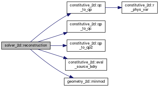
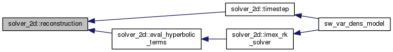
| subroutine solver_2d::reconstruction | ( | real*8, dimension(:,:,:), intent(in) | q_expl, |
| real*8, dimension(:,:,:), intent(in) | qp_expl | ||
| ) |
Linear reconstruction.
In this subroutine a linear reconstruction with slope limiters is applied to a set of variables describing the state of the system. In this way the values at the two sides of each cell interface are computed. This subroutine is also used for the boundary condition, when the reconstruction at the boundary interfaces are computed.
| [in] | q_expl | center values of the conservative variables |
| [in] | qp_expl | center values of the physical variables |
Definition at line 2486 of file solver_2d.f90.
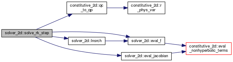
| subroutine solver_2d::solve_rk_step | ( | real*8, dimension(n_vars), intent(inout) | qj, |
| real*8, dimension(n_vars), intent(in) | qj_old, | ||
| real*8, dimension(n_rk), intent(in) | a_tilde, | ||
| real*8, dimension(n_rk), intent(in) | a_dirk, | ||
| real*8, intent(in) | a_diag | ||
| ) |
Runge-Kutta single step integration.
This subroutine find the solution of the non-linear system given the a step of the implicit-explicit Runge-Kutta scheme for a cell:

| [in,out] | qj | conservative variables |
| [in] | qj_old | conservative variables at the old time step |
| [in] | a_tilde | explicit coefficents for the fluxes |
| [in] | a_dirk | explicit coefficient for the non-hyperbolic terms |
| [in] | a_diag | implicit coefficient for the non-hyperbolic terms |
Definition at line 1228 of file solver_2d.f90.

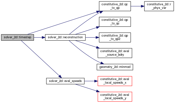
| subroutine solver_2d::timestep | ( | ) |
Time-step computation.
This subroutine evaluate the maximum time step according to the CFL condition. The local speed are evaluated with the characteristic polynomial of the Jacobian of the fluxes.
Definition at line 697 of file solver_2d.f90.
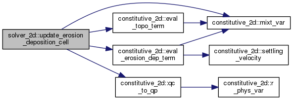
| subroutine solver_2d::update_erosion_deposition_cell | ( | real*8, intent(in) | dt | ) |
Evaluate the eroion/deposition terms.
This subroutine update the solution and the topography computing the erosion and deposition terms and the solution only because of entrainment.
| [in] | dt | time step |
Definition at line 1880 of file solver_2d.f90.
| real*8 solver_2d::a_diag |
Implicit coeff. for the non-hyp. part for a single step of the R-K scheme.
Definition at line 145 of file solver_2d.f90.
| real*8, dimension(:), allocatable solver_2d::a_dirk |
Explicit coeff. for the non-hyp. part for a single step of the R-K scheme.
Definition at line 142 of file solver_2d.f90.
| real*8, dimension(:,:), allocatable solver_2d::a_dirk_ij |
Butcher Tableau for the implicit part of the Runge-Kutta scheme.
Definition at line 130 of file solver_2d.f90.
| real*8, dimension(:,:,:), allocatable solver_2d::a_interface_x_max |
Max local speeds at the x-interface.
Definition at line 89 of file solver_2d.f90.
| real*8, dimension(:,:,:), allocatable solver_2d::a_interface_xneg |
Local speeds at the left of the x-interface.
Definition at line 95 of file solver_2d.f90.
| real*8, dimension(:,:,:), allocatable solver_2d::a_interface_xpos |
Local speeds at the right of the x-interface.
Definition at line 97 of file solver_2d.f90.
| real*8, dimension(:,:,:), allocatable solver_2d::a_interface_y_max |
Max local speeds at the y-interface.
Definition at line 91 of file solver_2d.f90.
| real*8, dimension(:,:,:), allocatable solver_2d::a_interface_yneg |
Local speeds at the bottom of the y-interface.
Definition at line 99 of file solver_2d.f90.
| real*8, dimension(:,:,:), allocatable solver_2d::a_interface_ypos |
Local speeds at the top of the y-interface.
Definition at line 101 of file solver_2d.f90.
| real*8, dimension(:), allocatable solver_2d::a_tilde |
Explicit coeff. for the hyperbolic part for a single step of the R-K scheme.
Definition at line 139 of file solver_2d.f90.
| real*8, dimension(:,:), allocatable solver_2d::a_tilde_ij |
Butcher Tableau for the explicit part of the Runge-Kutta scheme.
Definition at line 128 of file solver_2d.f90.
| real*8, dimension(:,:,:,:), allocatable solver_2d::divflux |
Intermediate hyperbolic terms of the Runge-Kutta scheme.
Definition at line 155 of file solver_2d.f90.
| real*8, dimension(:,:), allocatable solver_2d::divfluxj |
Local Intermediate hyperbolic terms of the Runge-Kutta scheme.
Definition at line 167 of file solver_2d.f90.
| real*8 solver_2d::dt |
Time step.
Definition at line 121 of file solver_2d.f90.
| real*8, dimension(:,:,:,:), allocatable solver_2d::expl_terms |
Intermediate explicit terms of the Runge-Kutta scheme.
Definition at line 164 of file solver_2d.f90.
| real*8, dimension(:,:), allocatable solver_2d::expl_terms_j |
Local Intermediate explicit terms of the Runge-Kutta scheme.
Definition at line 173 of file solver_2d.f90.
| real*8, dimension(:,:,:), allocatable solver_2d::h_interface_x |
Semidiscrete numerical interface fluxes.
Definition at line 103 of file solver_2d.f90.
| real*8, dimension(:,:,:), allocatable solver_2d::h_interface_y |
Semidiscrete numerical interface fluxes.
Definition at line 105 of file solver_2d.f90.
| integer solver_2d::i_rk |
loop counter for the RK iteration
Definition at line 125 of file solver_2d.f90.
| integer, dimension(:), allocatable solver_2d::j_cent |
Definition at line 190 of file solver_2d.f90.
| integer, dimension(:), allocatable solver_2d::j_stag_x |
Definition at line 193 of file solver_2d.f90.
| integer, dimension(:), allocatable solver_2d::j_stag_y |
Definition at line 196 of file solver_2d.f90.
| integer, dimension(:), allocatable solver_2d::k_cent |
Definition at line 191 of file solver_2d.f90.
| integer, dimension(:), allocatable solver_2d::k_stag_x |
Definition at line 194 of file solver_2d.f90.
| integer, dimension(:), allocatable solver_2d::k_stag_y |
Definition at line 197 of file solver_2d.f90.
| logical, dimension(:,:), allocatable solver_2d::mask11 |
Definition at line 123 of file solver_2d.f90.
| logical, dimension(:,:), allocatable solver_2d::mask12 |
Definition at line 123 of file solver_2d.f90.
| logical, dimension(:,:), allocatable solver_2d::mask21 |
Definition at line 123 of file solver_2d.f90.
| logical, dimension(:,:), allocatable solver_2d::mask22 |
Definition at line 123 of file solver_2d.f90.
| real*8, dimension(:,:,:,:), allocatable solver_2d::nh |
Intermediate non-hyperbolic terms of the Runge-Kutta scheme.
Definition at line 158 of file solver_2d.f90.
| real*8, dimension(:,:), allocatable solver_2d::nhj |
Local Intermediate non-hyperbolic terms of the Runge-Kutta scheme.
Definition at line 170 of file solver_2d.f90.
| logical solver_2d::normalize_f |
Flag for the normalization of the array f in the implicit solution scheme.
Definition at line 182 of file solver_2d.f90.
| logical solver_2d::normalize_q |
Flag for the normalization of the array q in the implicit solution scheme.
Definition at line 179 of file solver_2d.f90.
| real*8, dimension(:), allocatable solver_2d::omega |
Coefficients for the implicit part of the Runge-Kutta scheme.
Definition at line 136 of file solver_2d.f90.
| real*8, dimension(:), allocatable solver_2d::omega_tilde |
Coefficients for the explicit part of the Runge-Kutta scheme.
Definition at line 133 of file solver_2d.f90.
| logical solver_2d::opt_search_nl |
Flag for the search of optimal step size in the implicit solution scheme.
Definition at line 185 of file solver_2d.f90.
| real*8, dimension(:,:,:), allocatable solver_2d::q |
Conservative variables.
Definition at line 42 of file solver_2d.f90.
| real*8, dimension(:,:,:), allocatable solver_2d::q0 |
Conservative variables.
Definition at line 44 of file solver_2d.f90.
| real*8, dimension(:,:), allocatable solver_2d::q1max |
Maximum over time of thickness.
Definition at line 86 of file solver_2d.f90.
| real*8, dimension(:,:,:), allocatable solver_2d::q_cellne |
Reconstructed value at the NE corner of cell.
Definition at line 69 of file solver_2d.f90.
| real*8, dimension(:,:,:), allocatable solver_2d::q_cellnw |
Reconstructed value at the NW corner of cell.
Definition at line 67 of file solver_2d.f90.
| real*8, dimension(:,:,:), allocatable solver_2d::q_cellse |
Reconstructed value at the SE corner of cell.
Definition at line 73 of file solver_2d.f90.
| real*8, dimension(:,:,:), allocatable solver_2d::q_cellsw |
Reconstructed value at the SW corner of cell.
Definition at line 71 of file solver_2d.f90.
| real*8, dimension(:,:,:), allocatable solver_2d::q_fv |
Solution of the finite-volume semidiscrete cheme.
Definition at line 46 of file solver_2d.f90.
| real*8, dimension(:,:,:), allocatable solver_2d::q_interfaceb |
Reconstructed value at the bottom of the y-interface.
Definition at line 53 of file solver_2d.f90.
| real*8, dimension(:,:,:), allocatable solver_2d::q_interfacel |
Reconstructed value at the left of the x-interface.
Definition at line 49 of file solver_2d.f90.
| real*8, dimension(:,:,:), allocatable solver_2d::q_interfacer |
Reconstructed value at the right of the x-interface.
Definition at line 51 of file solver_2d.f90.
| real*8, dimension(:,:,:), allocatable solver_2d::q_interfacet |
Reconstructed value at the top of the y-interface.
Definition at line 55 of file solver_2d.f90.
| real*8, dimension(:,:,:,:), allocatable solver_2d::q_rk |
Intermediate solutions of the Runge-Kutta scheme.
Definition at line 148 of file solver_2d.f90.
| real*8, dimension(:,:,:), allocatable solver_2d::qp |
Physical variables ( )
Definition at line 107 of file solver_2d.f90.
| real*8, dimension(:,:,:), allocatable solver_2d::qp_cellne |
Reconstructed physical value at the NE corner of cell.
Definition at line 78 of file solver_2d.f90.
| real*8, dimension(:,:,:), allocatable solver_2d::qp_cellnw |
Reconstructed physical value at the NW corner of cell.
Definition at line 76 of file solver_2d.f90.
| real*8, dimension(:,:,:), allocatable solver_2d::qp_cellse |
Reconstructed physical value at the SE corner of cell.
Definition at line 82 of file solver_2d.f90.
| real*8, dimension(:,:,:), allocatable solver_2d::qp_cellsw |
Reconstructed physical value at the SW corner of cell.
Definition at line 80 of file solver_2d.f90.
| real*8, dimension(:,:,:), allocatable solver_2d::qp_interfaceb |
Reconstructed physical value at the bottom of the y-interface.
Definition at line 62 of file solver_2d.f90.
| real*8, dimension(:,:,:), allocatable solver_2d::qp_interfacel |
Reconstructed physical value at the left of the x-interface.
Definition at line 58 of file solver_2d.f90.
| real*8, dimension(:,:,:), allocatable solver_2d::qp_interfacer |
Reconstructed physical value at the right of the x-interface.
Definition at line 60 of file solver_2d.f90.
| real*8, dimension(:,:,:), allocatable solver_2d::qp_interfacet |
Reconstructed physical value at the top of the y-interface.
Definition at line 64 of file solver_2d.f90.
| real*8, dimension(:,:,:,:), allocatable solver_2d::qp_rk |
Intermediate physical solutions of the Runge-Kutta scheme.
Definition at line 151 of file solver_2d.f90.
| real*8, dimension(:,:,:), allocatable solver_2d::residual_term |
Sum of all the terms of the equations except the transient term.
Definition at line 188 of file solver_2d.f90.
| real*8, dimension(:,:,:,:), allocatable solver_2d::si_nh |
Intermediate semi-implicit non-hyperbolic terms of the Runge-Kutta scheme.
Definition at line 161 of file solver_2d.f90.
| real*8, dimension(:,:), allocatable solver_2d::si_nhj |
Local Intermediate semi-impl non-hyperbolic terms of the Runge-Kutta scheme.
Definition at line 176 of file solver_2d.f90.
| integer solver_2d::solve_cells |
Definition at line 116 of file solver_2d.f90.
| integer solver_2d::solve_interfaces_x |
Definition at line 117 of file solver_2d.f90.
| integer solver_2d::solve_interfaces_y |
Definition at line 118 of file solver_2d.f90.
| logical, dimension(:,:), allocatable solver_2d::solve_mask |
Definition at line 112 of file solver_2d.f90.
| logical, dimension(:,:), allocatable solver_2d::solve_mask_x |
Definition at line 113 of file solver_2d.f90.
| logical, dimension(:,:), allocatable solver_2d::solve_mask_y |
Definition at line 114 of file solver_2d.f90.
| real*8, dimension(:,:), allocatable solver_2d::source_xy |
Array defining fraction of cells affected by source term.
Definition at line 110 of file solver_2d.f90.
| real*8 solver_2d::t |
time
Definition at line 39 of file solver_2d.f90.
| real*8 solver_2d::t_imex1 |
Definition at line 199 of file solver_2d.f90.
| real*8 solver_2d::t_imex2 |
Definition at line 199 of file solver_2d.f90.
 1.8.11

